의사결정나무의 옵션 이해

의사결정나무의 여러 옵션들에 대해서 알아보자!

해당 포스트는 전북대학교 통계학과 최규빈 교수님의 강의내용을 토대로 재구성되었음을 알립니다.

1. 라이브러리 imports

import pandas as pd
import numpy as np
import matplotlib.pyplot as plt
import sklearn.tree
import graphviz

#-#
import warnings
warnings.filterwarnings('ignore')

2. max_features

(말그대로) 설명변수 몇 개 쓸거야???

# Data

df_train = pd.read_csv('https://raw.githubusercontent.com/guebin/MP2023/main/posts/insurance.csv')
df_train

	age	sex	bmi	children	smoker	region	charges
0	19	female	27.900	0	yes	southwest	16884.92400
1	18	male	33.770	1	no	southeast	1725.55230
2	28	male	33.000	3	no	southeast	4449.46200
3	33	male	22.705	0	no	northwest	21984.47061
4	32	male	28.880	0	no	northwest	3866.85520
...	...	...	...	...	...	...	...
1333	50	male	30.970	3	no	northwest	10600.54830
1334	18	female	31.920	0	no	northeast	2205.98080
1335	18	female	36.850	0	no	southeast	1629.83350
1336	21	female	25.800	0	no	southwest	2007.94500
1337	61	female	29.070	0	yes	northwest	29141.36030

1338 rows × 7 columns

# 적합 : max_features = 4

## step 1
X = pd.get_dummies(df_train.drop('charges', axis = 1), drop_first = True)
y = df_train.charges

## step 2
predictr = sklearn.tree.DecisionTreeRegressor(max_features = 4)

## step 3
predictr.fit(X, y)

DecisionTreeRegressor(max_features=4)

In a Jupyter environment, please rerun this cell to show the HTML representation or trust the notebook.
On GitHub, the HTML representation is unable to render, please try loading this page with nbviewer.org.

• 어떻게 적합했는지 프리 플랏으로 시각화하면…

sklearn.tree.plot_tree(predictr, max_depth = 0, feature_names = X.columns.to_list());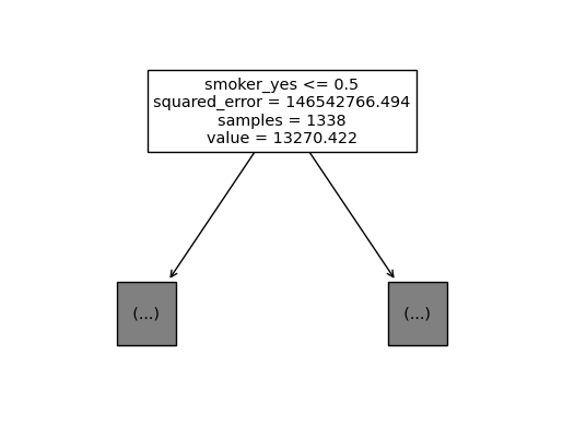

predictr.fit(X, y)
sklearn.tree.plot_tree(predictr, max_depth = 0, feature_names = X.columns.to_list());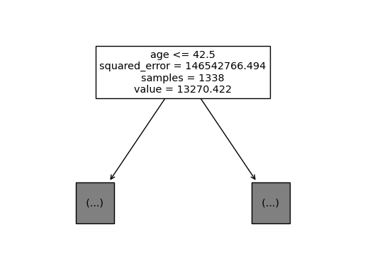

predictr.fit(X, y)
sklearn.tree.plot_tree(predictr, max_depth = 0, feature_names = X.columns.to_list());

max_features를 4로 제한했을 때, tree가 적합한 결과는 계속해서 달라진다.

len(X.columns)

8

max_features = 4의 의미는 설명변수들 중 4개만 임의로 뽑아서 그중 최적의 변수와 최적의 c를 찾겠다는 의미이다. (정말 가중치 없이 랜덤으로 막 뽑아버린다.)

이 경우는 smoker_yes가 가장 중요하여 이것이 뽑힌 절반 정도의 표본은 제일 위에 위치하게 된다.

3. random_state

모두 같은 결과를 보게 만들어 재현을 쉽게 하고 싶어!!

# 적합 : random_state = 42

## step 1
X = pd.get_dummies(df_train.drop('charges', axis = 1), drop_first = True)
y = df_train.charges

## step 2
predictr = sklearn.tree.DecisionTreeRegressor(max_features = 4, random_state = 42)

## step 3
predictr.fit(X, y)

DecisionTreeRegressor(max_features=4, random_state=42)

In a Jupyter environment, please rerun this cell to show the HTML representation or trust the notebook.
On GitHub, the HTML representation is unable to render, please try loading this page with nbviewer.org.

단순하다. train_test_split()이나, np.random.rand()나… 무작위로 뽑는 것에서 흔히 나타나는 random_state를 지정해주면 된다.

- 백날 돌려봐서 같은 결과가 나오는지 확인해보자.

graphviz.Source(sklearn.tree.export_graphviz(
    predictr,
    max_depth = 1,
    feature_names = X.columns.to_list()
))

predictr.fit(X, y)
graphviz.Source(sklearn.tree.export_graphviz(
    predictr,
    max_depth = 1,
    feature_names = X.columns.to_list()
))

아둔한 중생아… 몇 번을 시도해도 같은 결과가 나올 것이다…

4. .fit(sample_weight = [])

적합할 때에 사용하여 무게, 그러니까 가중치를 부여해주는 옵션이다. 특정 값을 중심으로 피팅을 해야 할 경우나, 값이 겹쳐있는 경우 유용한 옵션이다.

# 예제 1 아래의 데이터를 생각해보자.

X = np.array([1,2,3,4,5,6,7]).reshape(-1,1)
y = np.array([10,11,12,20,21,22,23])
plt.plot(X, y, 'o')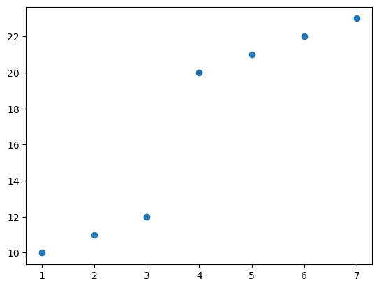

이것을 의사결정나무로 적합한다면 어떤 \(c\)값을 첫번째로 택해야 할까? \(\to\) 당연히 3.5정도가 되겠지…

predictr = sklearn.tree.DecisionTreeRegressor(max_depth = 1)
predictr.fit(X, y)
graphviz.Source(sklearn.tree.export_graphviz(predictr))

# 예제 2 유사하지만 다른 그림

## 점, 5000배.
X = np.array([1]*5000+[2]*5000+[3,4,5,6,7]).reshape(-1,1)
y = np.array([10]*5000+[11]*5000+[12,20,21,22,23])
plt.plot(X, y, 'o', alpha = 0.2)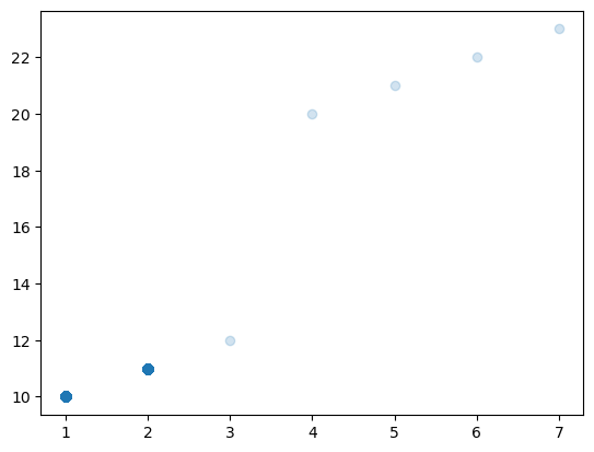

이 경우 산점도는 비슷하게 그려지지만, 1과 2에 5000개의 데이터들이 관측되었다. 따라서 1.5 근처에서 나누는 게 적합 점수가 높게 나올 것이다…

## 실제로 적합해보면...
predictr = sklearn.tree.DecisionTreeRegressor(max_depth = 1)
predictr.fit(X, y)
graphviz.Source(sklearn.tree.plot_tree(predictr));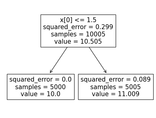

# 예제 3 가중치 부여

• 처음의 데이터를 이용했음에도, 위와 결과가 동일하도록 만들 수 있다.

X = np.array([1,2,3,4,5,6,7]).reshape(-1,1)
y = np.array([10,11,12,20,21,22,23])

plt.plot(X, y, 'o')
plt.plot(X[:2], y[:2], 'o')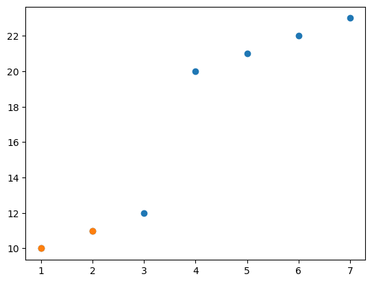

1번과 2번 데이터를 맞추는 것이 다른 것들보다 5000배 정도 더 중요하다면???~(중력, 5000배)~

predictr = sklearn.tree.DecisionTreeRegressor(max_depth = 1)
predictr.fit(X, y, sample_weight = [5000, 5000, 1,1,1,1,1])
graphviz.Source(sklearn.tree.export_graphviz(predictr))

이런 식으로 똑같은 결과를 볼 수 있다. 이 때, 샘플의 사이즈만 다르다.