import pandas as pd
import numpy as np
import matplotlib.pyplot as plt
import sklearn.linear_model범주형 반응변수의 예측 | LogisticRegression()
linear_model
예측해야 할 유형이 범주형일 때 사용할 수 있는 분석 기법 중 하나인 로지스틱 회귀분석을 해보자!
해당 포스트는 전북대학교 통계학과 최규빈 교수님의 강의내용을 토대로 재구성되었음을 알립니다.
1. 라이브러리 imports
2. 로지스틱 회귀분석
- 연속형 설명변수와 범주형 반응변수와의 관계
A. 성적과 취업 여부 데이터
- 학점과 토익 성적, 그리고 취업 여부를 나타낸 데이터가 있다.(교수님이 만드신 페이크 데이터이다.)
df = pd.read_csv('https://raw.githubusercontent.com/guebin/MP2023/main/posts/employment.csv')
df ## 페이크 데이터입니다.| toeic | gpa | employment | |
|---|---|---|---|
| 0 | 135 | 0.051535 | 0 |
| 1 | 935 | 0.355496 | 0 |
| 2 | 485 | 2.228435 | 0 |
| 3 | 65 | 1.179701 | 0 |
| 4 | 445 | 3.962356 | 1 |
| ... | ... | ... | ... |
| 495 | 280 | 4.288465 | 1 |
| 496 | 310 | 2.601212 | 1 |
| 497 | 225 | 0.042323 | 0 |
| 498 | 320 | 1.041416 | 0 |
| 499 | 375 | 3.626883 | 1 |
500 rows × 3 columns
plt.plot(df.toeic[df.employment == 0], df.gpa[df.employment == 0], 'o')
plt.plot(df.toeic[df.employment == 1], df.gpa[df.employment == 1], 'o')
plt.show()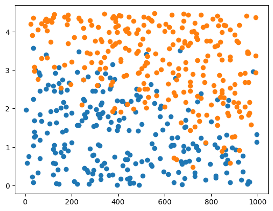
- 뭔가 관련성을 찾을 수 있을 것 같지 않은가?~(당연하지 그렇게 만드셨으니까)~
그래서 토익 성적ㆍ학점과 취업여부의 관계를 구하고 싶다.
### B. 분석
# step 1
X = pd.get_dummies(df[['toeic', 'gpa']])
y = df.employment

# step 2
predictr = sklearn.linear_model.LogisticRegression()

# step 3
predictr.fit(X, y)

# step 4
df = df.assign(employment_hat = predictr.predict(X))
sklearn.linear_model.LogisticRegression()
df| toeic | gpa | employment | employment_hat | |
|---|---|---|---|---|
| 0 | 135 | 0.051535 | 0 | 0 |
| 1 | 935 | 0.355496 | 0 | 0 |
| 2 | 485 | 2.228435 | 0 | 0 |
| 3 | 65 | 1.179701 | 0 | 0 |
| 4 | 445 | 3.962356 | 1 | 1 |
| ... | ... | ... | ... | ... |
| 495 | 280 | 4.288465 | 1 | 1 |
| 496 | 310 | 2.601212 | 1 | 0 |
| 497 | 225 | 0.042323 | 0 | 0 |
| 498 | 320 | 1.041416 | 0 | 0 |
| 499 | 375 | 3.626883 | 1 | 1 |
500 rows × 4 columns
로지스틱 회귀분석으로 적합 및 예측이 완료되었다.
C. 평가
predictr.score(X, y)0.882이건 y와 y_hat이 동일한 정도를 나타낸다, 나름 잘 맞춘 것 같지 않은가?
- 시각화를 해야 정확히 알 수 있겠지? 현재 예측치와 기존 예측치를 비교해보자.
df| toeic | gpa | employment | employment_hat | |
|---|---|---|---|---|
| 0 | 135 | 0.051535 | 0 | 0 |
| 1 | 935 | 0.355496 | 0 | 0 |
| 2 | 485 | 2.228435 | 0 | 0 |
| 3 | 65 | 1.179701 | 0 | 0 |
| 4 | 445 | 3.962356 | 1 | 1 |
| ... | ... | ... | ... | ... |
| 495 | 280 | 4.288465 | 1 | 1 |
| 496 | 310 | 2.601212 | 1 | 0 |
| 497 | 225 | 0.042323 | 0 | 0 |
| 498 | 320 | 1.041416 | 0 | 0 |
| 499 | 375 | 3.626883 | 1 | 1 |
500 rows × 4 columns
df_filtered = df[predictr.predict(X) == 1]

fig, (ax1, ax2) = plt.subplots(1, 2, figsize = (12,5))

fig.suptitle('Constrat Pradiction and Real')

ax1.plot(df.toeic, df.gpa, 'o', color = 'C0', label = 'employed')
ax1.plot(df.loc[df.employment == 1].toeic, df.loc[df.employment == 1].gpa, 'o', color = 'C1', label = 'not yet employed')
ax1.set_title('Real Data')

ax2.plot(df.toeic, df.gpa, 'o', color = 'C0', label = 'employed')
ax2.plot(df_filtered.toeic, df_filtered.gpa, 'o', color = 'C1', label = 'not yet employed')
ax2.set_title('Estimated Data')

plt.legend()
plt.show()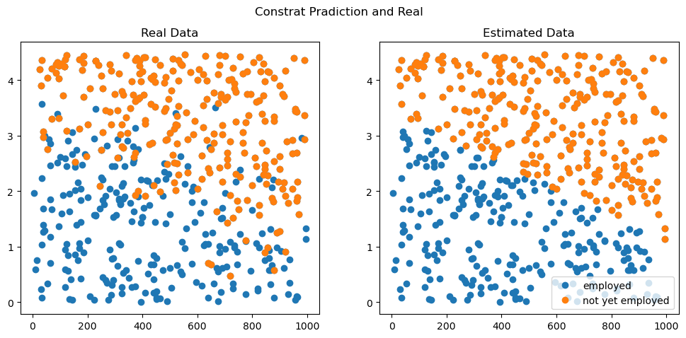
어때요, 나름 합리적이지 않나요?
3. 로지스틱 회귀분석의 실적용
그럼 타이타닉 데이터에서 로지스틱 회귀분석을 통해 결과를 잘 예측할 수 있지 않을까요?
df_train = pd.read_csv('https://raw.githubusercontent.com/HollyRiver/Machine_learning_in_practice/main/kaggle/titanic/data/train.csv')
df_test = pd.read_csv('https://raw.githubusercontent.com/HollyRiver/Machine_learning_in_practice/main/kaggle/titanic/data/test.csv')df_train.head()| PassengerId | Survived | Pclass | Name | Sex | Age | SibSp | Parch | Ticket | Fare | Cabin | Embarked | |
|---|---|---|---|---|---|---|---|---|---|---|---|---|
| 0 | 1 | 0 | 3 | Braund, Mr. Owen Harris | male | 22.0 | 1 | 0 | A/5 21171 | 7.2500 | NaN | S |
| 1 | 2 | 1 | 1 | Cumings, Mrs. John Bradley (Florence Briggs Th... | female | 38.0 | 1 | 0 | PC 17599 | 71.2833 | C85 | C |
| 2 | 3 | 1 | 3 | Heikkinen, Miss. Laina | female | 26.0 | 0 | 0 | STON/O2. 3101282 | 7.9250 | NaN | S |
| 3 | 4 | 1 | 1 | Futrelle, Mrs. Jacques Heath (Lily May Peel) | female | 35.0 | 1 | 0 | 113803 | 53.1000 | C123 | S |
| 4 | 5 | 0 | 3 | Allen, Mr. William Henry | male | 35.0 | 0 | 0 | 373450 | 8.0500 | NaN | S |
kaggle 입문하기에서 보았던 타이타닉 데이터이다.
- 여기서 반응변수를 쉽게 구하려면…
set(df_train.columns) - set(df_test.columns){'Survived'}- 하나만 남는 것을 볼 수 있다.
아! 테스트 셋에 없는 열이니까 저게 y겠구나!
### A. 늘 해왔던 것처럼 분석…~(하면 안된다)~
# step 1
X = pd.get_dummies(df_train.drop(['Survived'], axis = 1))
y = df_train.Survived
XX = pd.get_dummies(df_test)

# step 2
predictr = sklearn.linear_model.LogisticRegression()

# step 3
predictr.fit(X, y)
ValueError: Input X contains NaN.
LogisticRegression does not accept missing values encoded as NaN natively. For supervised learning, you might want to consider sklearn.ensemble.HistGradientBoostingClassifier and Regressor which accept missing values encoded as NaNs natively. Alternatively, it is possible to preprocess the data, for instance by using an imputer transformer in a pipeline or drop samples with missing values. See https://scikit-learn.org/stable/modules/impute.html You can find a list of all estimators that handle NaN values at the following page: https://scikit-learn.org/stable/modules/impute.html#estimators-that-handle-nan-values오류가 나온다.
Input X contains NaN.
선형 회귀에서 설명변수의 input값에는 결측치가 있으면 안된다!!!
df_train.info()<class 'pandas.core.frame.DataFrame'>
RangeIndex: 891 entries, 0 to 890
Data columns (total 12 columns):
# Column Non-Null Count Dtype
--- ------ -------------- -----
0 PassengerId 891 non-null int64
1 Survived 891 non-null int64
2 Pclass 891 non-null int64
3 Name 891 non-null object
4 Sex 891 non-null object
5 Age 714 non-null float64
6 SibSp 891 non-null int64
7 Parch 891 non-null int64
8 Ticket 891 non-null object
9 Fare 891 non-null float64
10 Cabin 204 non-null object
11 Embarked 889 non-null object
dtypes: float64(2), int64(5), object(5)
memory usage: 83.7+ KB결측치가 있는 열을 제거, 행을 제거, 둘 다. 또는 결측치를 impute해야 하는데…
- 일단 Cabin 열은 결측치가 너무 많으니까 빼자!
- Name이나 Ticket과 같은 변수는 이성적으로 봤을 때 바로 one-hot 인코딩 하기에는 어색하니 빼자!
len(set(df_train.Name)), len(set(df_train.Ticket)) ## 다 다름, 거의 다 다름(891, 681)- Age, Embarked에 포함된 약간의 결측치가 마음에 걸리니까 빼자!!
dropna() 메소드나 preprocessing을 써도 되지만… 그건 나중에 해보자.
df_test.info()<class 'pandas.core.frame.DataFrame'>
RangeIndex: 418 entries, 0 to 417
Data columns (total 11 columns):
# Column Non-Null Count Dtype
--- ------ -------------- -----
0 PassengerId 418 non-null int64
1 Pclass 418 non-null int64
2 Name 418 non-null object
3 Sex 418 non-null object
4 Age 332 non-null float64
5 SibSp 418 non-null int64
6 Parch 418 non-null int64
7 Ticket 418 non-null object
8 Fare 417 non-null float64
9 Cabin 91 non-null object
10 Embarked 418 non-null object
dtypes: float64(2), int64(4), object(5)
memory usage: 36.0+ KB- Fare에 포함된 결측치도 걸린다 -> 빼자! (평균으로 해주는 방법도 있는ㄷ ~나중에 하자고 좀~)
B. 데이터 정리
- 위에서 말한 조건들을 적용해서 데이터를 재가공한 뒤, 로지스틱 회귀를 해보자
df_train.columnsIndex(['PassengerId', 'Survived', 'Pclass', 'Name', 'Sex', 'Age', 'SibSp',
'Parch', 'Ticket', 'Fare', 'Cabin', 'Embarked'],
dtype='object')# step 1
X = pd.get_dummies(df_train.drop(['Survived', 'Cabin', 'Name', 'Ticket', 'Age', 'Embarked', 'Fare'], axis = 1))
y = df_train.Survived
XX = pd.get_dummies(df_test.drop(['Cabin', 'Name', 'Ticket', 'Age', 'Embarked', 'Fare'], axis = 1))
# step 2
predictr = sklearn.linear_model.LogisticRegression()
# step 3
predictr.fit(X, y)
# step 4
XX.assign(Survived = predictr.predict(XX))| PassengerId | Pclass | SibSp | Parch | Sex_female | Sex_male | Survived | |
|---|---|---|---|---|---|---|---|
| 0 | 892 | 3 | 0 | 0 | False | True | 0 |
| 1 | 893 | 3 | 1 | 0 | True | False | 1 |
| 2 | 894 | 2 | 0 | 0 | False | True | 0 |
| 3 | 895 | 3 | 0 | 0 | False | True | 0 |
| 4 | 896 | 3 | 1 | 1 | True | False | 1 |
| ... | ... | ... | ... | ... | ... | ... | ... |
| 413 | 1305 | 3 | 0 | 0 | False | True | 0 |
| 414 | 1306 | 1 | 0 | 0 | True | False | 1 |
| 415 | 1307 | 3 | 0 | 0 | False | True | 0 |
| 416 | 1308 | 3 | 0 | 0 | False | True | 0 |
| 417 | 1309 | 3 | 1 | 1 | False | True | 0 |
418 rows × 7 columns
정상적으로 잘 수행한 것 같다.
### C. 평가
predictr.score(X, y)0.8002244668911336생각보단 잘 한 것 같다.
D. 제출
yy = pd.DataFrame({'Survived' : predictr.predict(XX)})
submit_df = pd.concat([df_test.PassengerId, yy], axis = 1)
submit_df

#submit_df.to_csv(directory, index = False)| PassengerId | Survived | |
|---|---|---|
| 0 | 892 | 0 |
| 1 | 893 | 1 |
| 2 | 894 | 0 |
| 3 | 895 | 0 |
| 4 | 896 | 1 |
| ... | ... | ... |
| 413 | 1305 | 0 |
| 414 | 1306 | 1 |
| 415 | 1307 | 0 |
| 416 | 1308 | 0 |
| 417 | 1309 | 0 |
418 rows × 2 columns
kaggle에 제출하고 두근대는 결과는… 0.77511, 그리 높진 않다.