import matplotlib.pyplot as plt
import numpy as np
import matplotlib
matplotlib.rcParams['figure.figsize'] = (3, 2)
matplotlib.rcParams['figure.dpi'] = 150Plot | 꺾은선, 산점도, 객체지향화
matplotlib
matplotlib를 이용하여 그래프를 그려보자!
해당 포스트는 전북대학교 통계학과 최규빈 교수님의 강의내용을 토대로 재구성되었음을 알립니다.
1. 사전작업
- 라이브러리 import
2. 간단한 꺾은선 그래프
plt.plot()을 사용하여 간단하게 그래프를 그릴 수 있다.
- y값만 지정한 경우
plt.plot([1,2,4,3])
plt.show()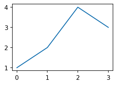
- x값과 y값 같이 지정한 경우
plt.plot([1,2,3,4],[1,2,4,3])
plt.show()
- x값과 y값에 변수를 지정하여 넣어주는 경우
x = [1,2,3,4]
y = [1,2,4,3]

plt.plot(x,y)
plt.show()
- 이외에도 다양한 옵션을 사용하여 그래프를 다채롭게 그릴 수 있는데, 지금부터 그것들을 알아보도록 하자.
plt.plot의 옵션
plt.plot()에서 괄호 안에 문자열을 넣음으로서 세 가지 옵션을 간단하게 적용할 수 있다.
plt.plot(x,y,'--')  ## 파선 그래프
plt.plot(x,y,':')   ## 점선 그래프
plt.plot(x,y,'r')   ## 선의 색상이 빨간색
plt.plot(x,y,'r--') ## 빨간색의 파선 그래프
...
- 게다가 세 옵션을 순서 상관없이 집어넣어 적용 가능하다!
| character | description |
|---|---|
| ‘-’ | solid line style |
| ‘–’ | dashed line style |
| ‘-.’ | dash-dot line style |
| ‘:’ | dotted line style |
| character | color |
|---|---|
| ‘b’ | blue |
| ‘g’ | green |
| ‘r’ | red |
| ‘c’ | cyan |
| ‘m’ | magenta |
| ‘y’ | yellow |
| ‘k’ | black |
| ‘w’ | white |
| character | description |
|---|---|
| ‘.’ | point marker |
| ‘,’ | pixel marker |
| ‘o’ | circle marker |
| ‘v’ | triangle_down marker |
| ‘^’ | triangle_up marker |
| ‘<’ | triangle_left marker |
| ‘>’ | triangle_right marker |
| ‘1’ | tri_down marker |
| ‘2’ | tri_up marker |
| ‘3’ | tri_left marker |
| ‘4’ | tri_right marker |
| ‘8’ | octagon marker |
| ‘s’ | square marker |
| ‘p’ | pentagon marker |
| ‘P’ | plus (filled) marker |
| ’*’ | star marker |
| ‘h’ | hexagon1 marker |
| ‘H’ | hexagon2 marker |
| ‘+’ | plus marker |
| ‘x’ | x marker |
| ‘X’ | x (filled) marker |
| ‘D’ | diamond marker |
| ‘d’ | thin_diamond marker |
| ‘|’ | vline marker |
| ’_’ | hline marker |
그 외에 다른 옵션을 보고 싶다면 아래를 참조하라.
other options or colors
https://matplotlib.org/stable/api/_as_gen/matplotlib.pyplot.plot.html
https://matplotlib.org/2.0.2/examples/color/named_colors.html
hex code
https://htmlcolorcodes.com/
other linestyles
https://matplotlib.org/stable/gallery/lines_bars_and_markers/linestyles.html
- preset에 있는 색상 외 다른 색상을 적용
plt.plot(x,y,'--',color = 'lime')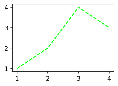
using color name
plt.plot(x,y,color = '#751F9B')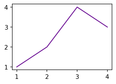
using hex code
- 선의 형태를 다양하게 변경
plt.plot(x,y,linestyle = 'dashed')
plt.show()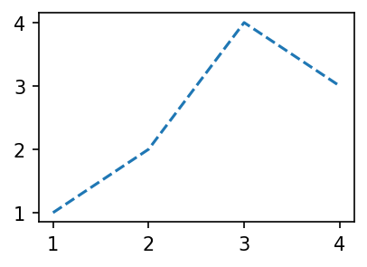
문자열로 직접 지정
plt.plot(x,y,linestyle = (0, (1,1)))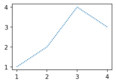
파선의 길이를 직접 지정
plt.plot()에서 scatter plot을 생성
marker 옵션을 변경하여 scatter plot을 손쉽게 그릴 수도 있다.
plt.plot(x,y,'db') ## diamonds, blue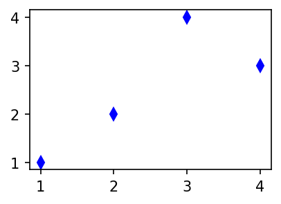
dot connected plot
plt.plot(x,y,':or') ## dotline(:), circle(o), red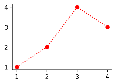
pile up
plt.show()를 입력하기 전 계속해서 그래프를 그리면 중첩된다.
plt.plot([1,2,3,2], '--o', color = 'orange')
plt.plot([2,3,1,4], '--o', color = 'skyblue')
plt.show()
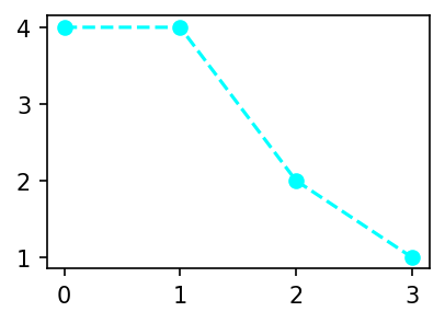
plt.plot([4,4,2,1], '--o', color = 'cyan')
plt.show()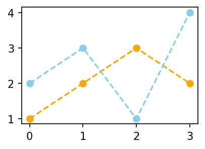
plt.plot([1,2,3,2], '--o', color = 'C1')
plt.plot([2,3,1,4], '--o', color = 'C0')

plt.show()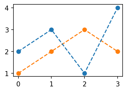
위와 같은 경우에는 color를 지정하지 않을 경우 먼저 입력한 그래프에 C0가 지정된다.
응용 : scatter plot and line plot
- 유사 단순선형회귀
설명변수와 오차, 반응변수를 지정해주자.
x = np.arange(-5,5,0.1)
eps = np.random.randn(100)
y = 2*x + eps ## 벗어나도록 겹치게plt.plot(x,y,'.b') ## 실제 데이터
plt.plot(x,2*x,'--r') ## 회귀선
plt.show()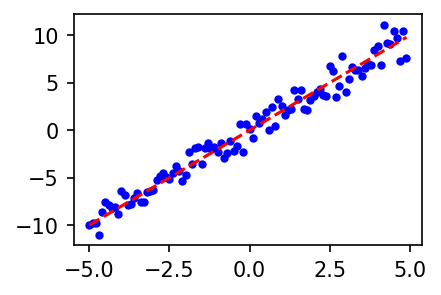
적합한 그래프를 그릴 때
- summary: boxplot, histogram, lineplot, scatterplot
- 라인플랏: 추세
- ☆★☆ 스캐터플랏: 두 변수의 관계
- 박스플랏: 분포(일상용어)의 비교, 이상치
- 히스토그램: 분포(통계용어)파악
- 바플랏: 크기비교
3. 객체지향적 시각화
A. 배경지식
- 그림을 저장해둔 뒤 나중에 꺼내보고 싶다면? | plt.gcf() : Get Current Figure.
plt.plot([1, 2, 3, 2],'--o')
fig = plt.gcf() ## plt.show()를 하기 전, 현재 표기되는 figure를 얻는다.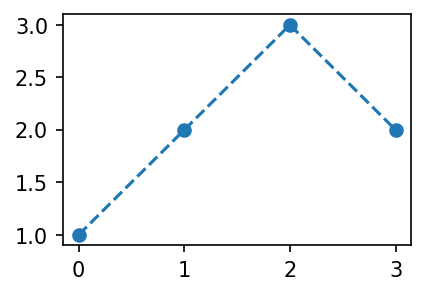
fig
위와 같이 변수에 저장된 것을 알 수 있다.
B. fig의 해체
fig
fig.axes

ax = fig.axes[0]
ax.yaxis
ax.xaxis

lines = ax.get_lines()[0]
lines[0]- fig > 그래프 그 자체
- axes > 그래프의 구역
- axis > x축, y축
- line > 직선형 그래프
등등등…
아무튼 여러 개체가 나뉘어있다.
개념(비유) : * Figure(fig) : 도화지 * Axes(ax) : 도화지에 존재하는 그림틀 * Axis, Lines : 그림틀 위에 올려지는 물체(object)
C. plt.plot()없이 그래프 그리기
plt.plot([1,2,4,3], '--o')
plt.show()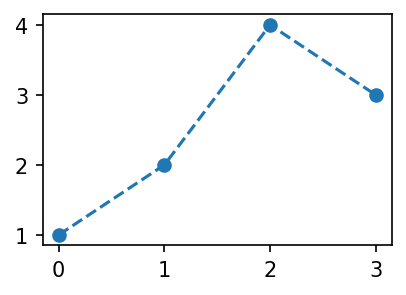
위와 같은 그래프를 plt.plot()없이 만들어보자!
- 아래의 코드를 하나하나 뜯어보자.
fig = plt.Figure()

ax = fig.add_axes([0.125,0.11,0.775,0.77])
ax.set_xlim([-0.15, 3.15])  # setting x axis limit
ax.set_ylim([0.9, 3.1])     # setting y axis limit
line = matplotlib.lines.Line2D(
    xdata = [0,1,2,3],
    ydata = [1,2,3,2],
    linestyle = '--',
    marker = 'o'
)
ax.add_line(line)

fig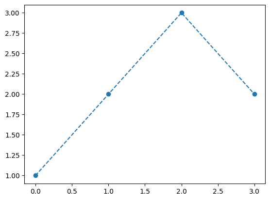
1. 최상위 하이라이트(figure) 생성
fig = plt.figure(); fig ## 최상위 하이라이트인 그림만 만들어냄.<Figure size 450x300 with 0 Axes><Figure size 450x300 with 0 Axes>2. 그래프가 들어갈 공간(axes) 생성
ax = fig.add_axes([0.125,0.11,0.775,0.77]); fig ## 가로시작, 세로시작, 종횡비
3. 직선을 지정 후 추가
line = matplotlib.lines.Line2D(
    xdata = [0,1,2,3],
    ydata = [1,2,3,2],
    linestyle = '--',
    marker = 'o'
)
matplotlib에서 라인을 만드는 함수가 따로 있었다.
ax.add_line(line)fig
4. 직선이 제대로 표기되지 않는 것 같으니 x축과 y축의 한계를 설정
ax.set_xlim([-0.15, 3.15])
ax.set_ylim([0.9, 3.1])

fig
D. 또 코드의 대체
1. line2D 오브젝트를 쓰지 않는 방법
## genarally
fig = plt.Figure()
ax = fig.add_axes([0.125, 0.11, 0.775, 0.77])
ax.plot([1,2,3,2], '--o')
fig
ax.plot()을 사용
2. add_axes()를 쓰지 않는 방법(중요!)
fig = plt.Figure()
ax = fig.subplots(1)
ax.plot([1,2,3,2], '--o')
fig
ax = fig.subplots()을 사용
3. fig와 ax들을 한번에 지정(중요!)
fig, ax = plt.subplots(1) ## 중요함
ax.plot([1,2,3,2], '--o')
plt.show()
E. 정리 (\(\star\star\star\))
아래의 코드는 모두 같은 애들이었다.
plt.plot([1,2,3,2], '--o')
fig, ax = plt.subplots()
ax.plot([1,2,3,2], '--o')
fig = plt.Figure()
ax = fig.subplots()
ax.plot([1,2,3,2], '--o')
fig
fig = plt.Figure()
ax = fig.add_axes([0.125, 0.11, 0.775, 0.77])
ax.plot([1,2,3,2], '--o')
fig
plt.subplots()과 ax.plot()의 경우 상당히 유용한 코드이니 꼭 숙지할 것!
4. 미니맵과 서브플롯
A. 미니맵
fig.add_axes()를 사용한다.
fig = plt.Figure()
ax = fig.add_axes([0,0,2,2]); fig
ax_mini = fig.add_axes([1.4,0.2,0.5,0.5])  ## 가로 세로 위치(중심위치), 종횡비
ax.plot([1,5,3,4], '--o')
ax_mini.plot([1,2,3,1], '--or')

fig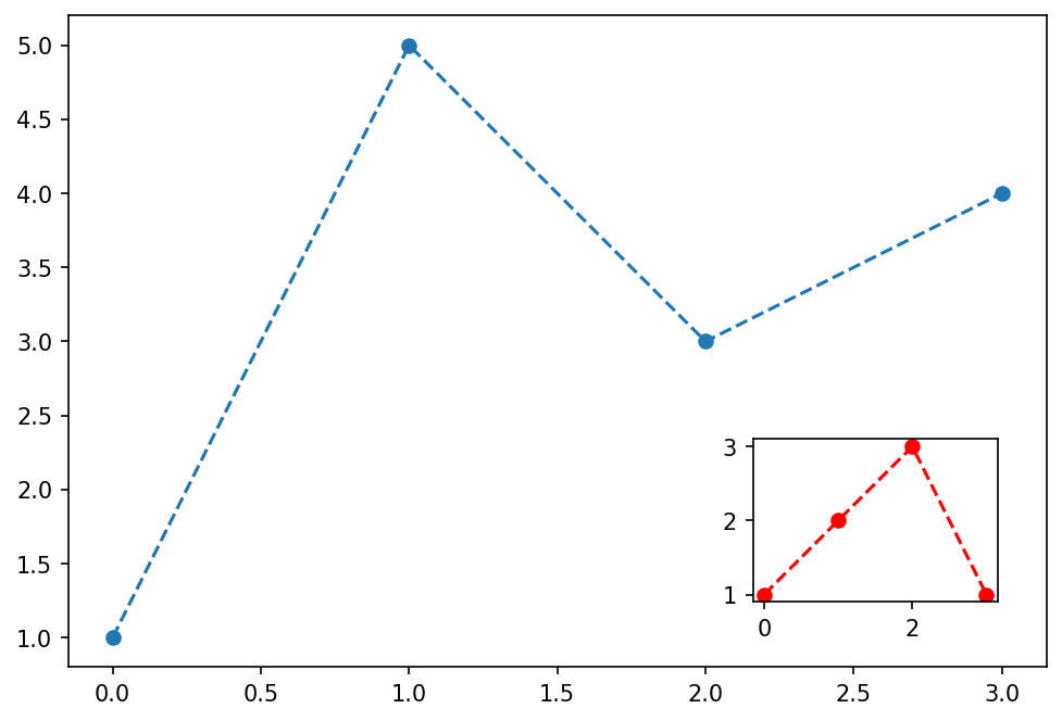
생성된 fig에 axes를 하나 더 추가하여 만들어냈다.
B. 서브플롯
plt.subplots(), fig.subplots()을 이용해보자.
fig, axs = plt.subplots(2) ## 2행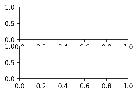
axsarray([<AxesSubplot:>, <AxesSubplot:>], dtype=object)
axs에ax들이array형태로 저장되어 있다.
axs[0].plot([1,2,3,2], '--r')
axs[1].plot([1,2,4,3], '--o')

fig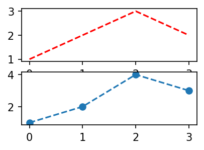
뭔가 레이아웃이 가려져있고 이상하다.
fig.tight_layout(); fig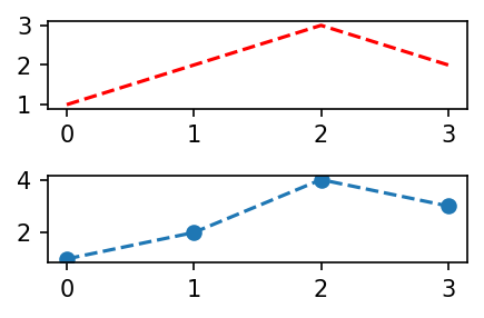
왠만해선
fig.tight_layout()을 해주도록 하자.
- 차피 axs가 array 형태로 저장되므로 그것을 따로 지정해주고 싶다면 아래와 같이 사용하는 것을 권장한다.
fig, (ax1, ax2) = plt.subplots(2)
ax1.plot([1,2,3,2], '--r')
ax2.plot([1,2,4,3], '--o')
fig.tight_layout()
C. 서브플롯 스케일 조정 및 다중화
- 스케일 변경
fig, (ax1, ax2) = plt.subplots(2, figsize = (3,3))  ## 종횡비
ax1.plot([1,2,3,2], '--r')
ax2.plot([1,2,4,3], '--o')
fig.tight_layout()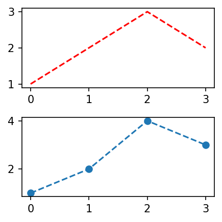
미리 설정해줬던 dpi에 의거하여 종횡비가 배수로 적용된다.
- 더 많은 서브플롯 생성
fig, ((ax1, ax2),(ax3,ax4)) = plt.subplots(2,2, figsize = (3,3))
ax1.plot([1,2,4,3], 'o', color = 'C0')
ax2.plot([1,2,4,3], 'o', color = 'C1')
ax3.plot([1,2,4,3], 'o', color = 'C2')
ax4.plot([1,2,4,3], 'o', color = 'C3')
fig.tight_layout()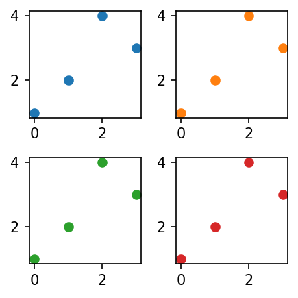
- 사용자 정의 서브플롯 생성
plt.subplot() ## s가 없는 subplot(), 즉, 하나만 만들어진다.
plt.figure(figsize=(3,3))
plt.subplot(2,2,1)  ## 2×2의 1
plt.plot([1,2,4,3],'o', color='C0')
plt.subplot(1,2,2)
plt.plot([1,2,4,3],'o', color='C1')
plt.subplot(2,2,3)
plt.plot([1,2,4,3],'o', color='C2')
plt.tight_layout()

fig = plt.gcf()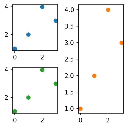
- 이미 생성된 figure의 크기를 조정
fig.set_size_inches(2,2); fig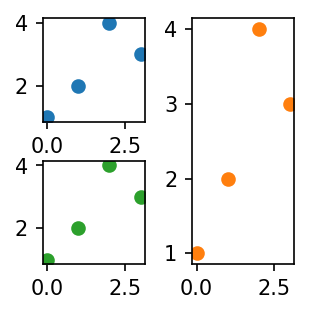
5. title
title을 만드는 함수는 어떤 오브젝트에 소속되는 게 좋을까? 1. plt -> subplot의 제목을 설정 가능 2. fig -> 전체제목(super title)을 설정할 수 있음 3. ax -> subplot들의 제목을 설정할 수 있음
A. plt.title()
figure를 생성하지 않은 기본적인 환경에서 타이틀을 달아준다.
## 가장 평범한 플롯
plt.plot([1,2,3,2])
plt.title('asdf')
plt.show()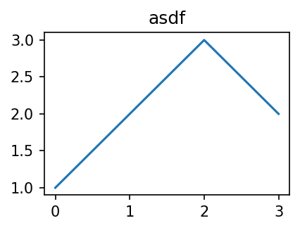
B. ax.set_title()
figure와 axes를 생성했을 경우, 각 ax마다 타이틀을 달아줄 수 있다.
## title이 axes에 존재
fig, ax = plt.subplots()
ax.set_title('asdf')
ax.plot([1,2,3,2])

plt.show()
C. fig.suptitle() | 권장하지 않는 방법
원래 figure 자체에 타이틀을 붙이는 것은 불가능하다.
##--------fig : 원래는 불가능--------
plt.plot([1,2,3,2])
fig = plt.gcf()
fig.suptitle('asdf')

plt.show()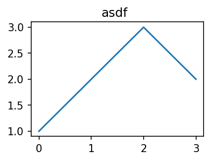
D. 응용
plt.subplots()과set_title()을 이용
fig, (ax1, ax2) = plt.subplots(1,2, figsize = (4,2))
ax1.set_title('asdf')
ax2.set_title('1234')
ax1.plot([1,2,3,2])
ax2.plot([1,2,3,2])
fig.tight_layout()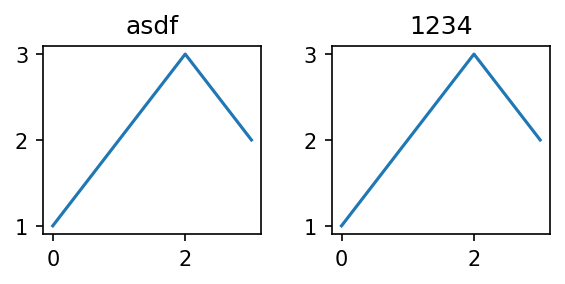
- figure를 생성하지 않고
plt.subplot()과plt.title()을 이용하여 손수 지정
plt.subplot(1,2,1)
plt.plot([1,2,3])
plt.title('asdf')
plt.subplot(1,2,2)
plt.plot([1,2,3])
plt.title('1234')
plt.tight_layout()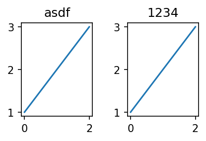
fig.suptitle()을 이용한 방법
fig, (ax1, ax2) = plt.subplots(1,2)
ax1.set_title('asdf')
ax2.set_title('1234')
fig.suptitle('asdf1234')
fig.tight_layout()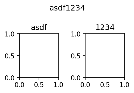
E. plt.gca()
plt.gca()를 통해 ax개체를 다룰 수도 있다.
plt.plot([1,2,3,2])
ax = plt.gca()
ax.set_title('asdf')  ## 현재의 axis에 바로 타이틀을 설정해준다.
Text(0.5, 1.0, 'asdf')
6. 산점도의 응용 | 표본상관계수
A. 산점도와 표본상관계수
아래처럼 두 연속형 자료가 주어질 경우 산점도로 나타낼 수 있다.
weight = [44,48,49,58,62,68,69,70,76,79]
height = [159,160,162,165,167,162,165,175,165,172]

plt.plot(weight,height,'.')  ## option : '.' marker가 .인 산점도 산출
plt.show()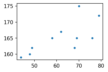
아래 표본상관계수의 정의에 따라 데이터에서의 표본상관계수를 구해보자.
- (표본)상관계수의 정의
\[r=\frac{\sum_{i=1}^{n}(x_i-\bar{x})(y_i-\bar{y}) }{\sqrt{\sum_{i=1}^{n}(x_i-\bar{x})^2\sum_{i=1}^{n}(y_i-\bar{y})^2 }}=\sum_{i=1}^{n}\tilde{x}_i\tilde{y}_i \]
\[단,~\tilde{x}_i=\frac{(x_i-\bar{x})}{\sqrt{\sum_{i=1}^n(x_i-\bar{x})^2}},~ \tilde{y}_i=\frac{(y_i-\bar{y})}{\sqrt{\sum_{i=1}^n(y_i-\bar{y})^2}}\]
위 식에서 \(\tilde{x}_i\)와 \(\tilde{y}_i\)는 \(x_i\)와 \(y_i\)를 표준화한 것이다.
(데이터를 불러오자)
x=[44,48,49,58,62,68,69,70,76,79]
y=[159,160,162,165,167,162,165,175,165,172]
(평균을 0으로)
xx = x - np.mean(x); print(xx)
yy = y - np.mean(y); print(yy)
[-18.3 -14.3 -13.3 -4.3 -0.3 5.7 6.7 7.7 13.7 16.7]
[-6.2 -5.2 -3.2 -0.2 1.8 -3.2 -0.2 9.8 -0.2 6.8](퍼진 정도를 표준화)
x_standard = xx/np.sqrt(np.sum(xx**2))
y_standard = yy/np.sqrt(np.sum(yy**2))
(표본상관계수 산출)
np.sum(x_standard*y_standard)0.7138620583559141- 이미 정의된 코드를 통해 해당 결과가 맞는지 확인해보자.
np.corrcoef(x,y)array([[1. , 0.71386206],
[0.71386206, 1. ]])### B. 산점도를 보고 상관계수의 부호를 해석
- 아래의 그림은 상관계수 r의 값이 양수인가 음수인가?
x=[44,48,49,58,62,68,69,70,76,79]
y=[159,160,162,165,167,162,165,175,165,172]

plt.plot(x, y, 'o')
plt.show()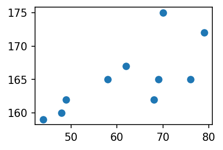
xx = x-np.mean(x)
yy = y-np.mean(y)
xxx = xx/np.sqrt(np.sum(xx**2))
yyy = yy/np.sqrt(np.sum(yy**2))
fig, (ax1, ax2, ax3) = plt.subplots(1,3, figsize = (10,3))
ax1.plot(x,y, 'o')
ax1.set_title(r'$(x_i,y_i)$')
ax2.plot(xx,yy,'o') ## mean to 0
ax2.set_title(r'$(x_i-\bar{x}, y_i-\bar{y})$')
ax3.plot(xxx,yyy,'o') ## standarized
ax3.set_title(r'$(\tilde{x}_i,\tilde{y}_i)$')
plt.show()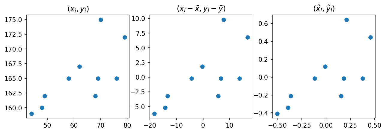
- 마지막 \(\tilde{x}_i\), \(\tilde{y}_i\)를 곱한 값이 양수인 것과 음수인 것을 체크해보자.
1,3사분면에 점들이 많으므로 상관계수의 부호는 양수일 것이다.
### D. 산점도를 보고 상관계수의 절대값을 해석
- 기울기가 동일하지만 직선 근처의 퍼짐이 다른 두 개의 자료
x=np.arange(0,10,0.1)
y1=x+np.random.normal(loc=0,scale=1.0,size=len(x))  ## N(0,1)
y2=x+np.random.normal(loc=0,scale=7.0,size=len(x))  ## N(0,7)

plt.plot(x,y1,'.')
plt.plot(x,y2,'x')
plt.show()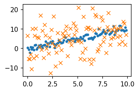
- 표준화하는 함수
tilde()정의
def tilde(x):
    xx = x-np.mean(x)
    xxx = xx / np.sqrt(np.sum(xx**2))
    return xxx
fig, (ax1, ax2) = plt.subplots(1,2, figsize = (4,2))
ax1.plot(x,y1,'.'); ax1.plot(x,y2,'x'); ax1.set_title(r'$(x_i,y_i)$')
ax2.plot(tilde(x), tilde(y1),'.'); ax2.plot(tilde(x), tilde(y2), 'x'); ax2.set_title(r'$(\tilde{x}_i,\tilde{y}_i)$')
fig.tight_layout()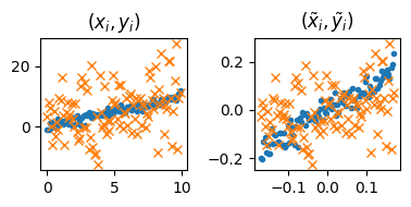
- 직선 근처의 퍼짐은 동일하지만, 직선의 기울기가 다른 경우
x=np.arange(0,10,0.1)
y1=x+np.random.normal(loc=0,scale=1.0,size=len(x))  ## 기울기가 1
y2=0.2*x+np.random.normal(loc=0,scale=1.0,size=len(x))  ## 기울기가 0.2

plt.plot(x,y1,'.')
plt.plot(x,y2,'x')

plt.show()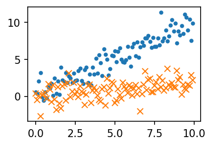
fig, (ax1,ax2) = plt.subplots(1,2,figsize=(4,2))
ax1.plot(x,y1,'.'); ax1.plot(x,y2,'x'); ax1.set_title(r'$(x_i,y_i)$')
ax2.plot(tilde(x),tilde(y1),'.'); ax2.plot(tilde(x),tilde(y2),'x'); ax2.set_title(r'$(\tilde{x}_i,\tilde{y}_i)$')
fig.tight_layout()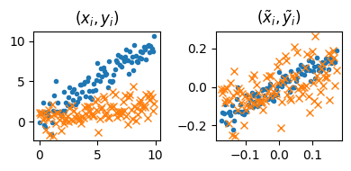
기울기가 클수록, 퍼짐 정도가 작을수록 상관계수의 절댓값이 높다.
7. 산점도 응용예제2 - 앤스콤의 4분할
- 표본상관계수가 모두 동일한 네 자료를 보라.
x1 = [10, 8, 13, 9, 11, 14, 6, 4, 12, 7, 5]
y1 = [8.04, 6.95, 7.58, 8.81, 8.33, 9.96, 7.24, 4.26, 10.84, 4.82, 5.68]

x2 = x1
y2 = [9.14, 8.14, 8.74, 8.77, 9.26, 8.10, 6.13, 3.10, 9.13, 7.26, 4.74]

x3 = x1
y3 = [7.46, 6.77, 12.74, 7.11, 7.81, 8.84, 6.08, 5.39, 8.15, 6.42, 5.73]

x4 = [8, 8, 8, 8, 8, 8, 8, 19, 8, 8, 8]
y4 = [6.58, 5.76, 7.71, 8.84, 8.47, 7.04, 5.25, 12.50, 5.56, 7.91, 6.89]

np.corrcoef(x1,y1),np.corrcoef(x2,y2),np.corrcoef(x3,y3),np.corrcoef(x4,y4)
(array([[1. , 0.81642052],
[0.81642052, 1. ]]),
array([[1. , 0.81623651],
[0.81623651, 1. ]]),
array([[1. , 0.81628674],
[0.81628674, 1. ]]),
array([[1. , 0.81652144],
[0.81652144, 1. ]]))음, 다 비슷한 자료겠구나… 양의 상관관계를 띄겠네?
라고 속단하긴 이르다.
fig, ((ax1,ax2),(ax3,ax4)) = plt.subplots(2,2,figsize=(6,4))
ax1.plot(x1,y1,'o'); ax1.set_title(f'corrcoef = {np.corrcoef(x1,y1)[0,1] : .6f}')
ax2.plot(x2,y2,'o'); ax2.set_title(f'corrcoef = {np.corrcoef(x2,y2)[0,1] : .6f}')
ax3.plot(x3,y3,'o'); ax3.set_title(f'corrcoef = {np.corrcoef(x3,y3)[0,1] : .6f}')
ax4.plot(x4,y4,'o'); ax4.set_title(f'corrcoef = {np.corrcoef(x4,y4)[0,1] : .6f}')
fig.tight_layout()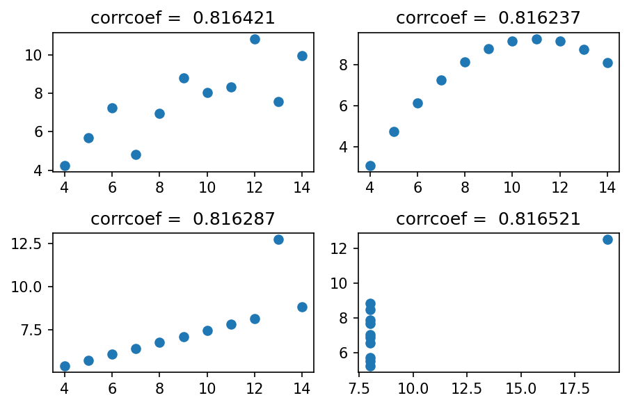
4개의 그림은 모두 같은 상관계수를 가지나, 그 느낌이 전혀 다르다.
- 앤스콤플랏의 4개의 그림은 모두 같은 상관계수를 가진다. 하지만, 4개의 그림은 느낌이 전혀 다르다.
- 같은 표본상관계수를 가진다고 하여 같은 관계성을 가지는 것은 아니다. 표본상관계수는 x,y의 비례정도를 측정하는데 그 값이 1에 가깝다고 하여 꼭 정비례의 관계가 있음을 의미하는 건 아니다.
\((x_i,y_i)\)의 산점도가 선형성을 보일 때만 “표본상관계수가 1에 가까우므로 정비례의 관계에 있다”라는 논리전개가 성립한다.
- 앤스콤의 첫번째 플랏 : 산점도가 선형 -> 표본상관계수가 0.816 = 정비례의 관계가 0.816 정도
- 앤스콤의 두번째 플랏 : 산점도가 선형이 아님 -> 표본상관계수가 크게 의미없음.
- 앤스콤의 세번째 플랏 : 산점도가 선형인듯 보이나 하나의 이상치가 있음 -> 하나의 이상치가 표본상관계수의 값을 무너뜨릴 수 있으므로 표본상관계수 값을 신뢰할 수 없음.
- 앤스콤의 네번째 플랏 : 산점도를 그려보니 이상한 그림 -> 표본상관계수를 계산할 수는 있으나, 그게 무슨 의미가 있을까?
산점도가 선형성을 보일 때만 표본상관계수가 1에 가까우므로 정비례의 관계에 있다라는 논리전개가 성립한다.
1번만 의미가 있음. 3번의 경우 이상치가 존재하여 신뢰할 수 없음.
교훈
상관계수를 해석하기에 앞서서 산점도가 선형성을 보이는 지 체크할 것! 항상 통계량은 적절한 가정하에서만 말이 된다는 사실을 기억할 것!